Life Cycle Cost Modelling

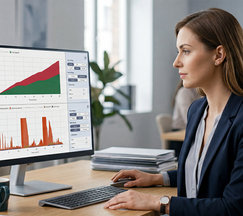
Life cycle cost modeling is the structured method for building a model of a system’s total cost over its whole life, from research and development through procurement, operating and support, and disposal. With Opus Suite+, program teams link each cost to its technical drivers and compare alternatives on total cost of ownership.

Life cycle cost modeling is the structured method for building a model of a system's total cost over its whole life, from research and development through procurement, operating and support, and disposal. An LCC model links each cost to the technical and operational drivers behind it, such as reliability, maintenance concept and operating tempo. Program teams use it to compare design options, support concepts and acquisition strategies on total cost of ownership rather than purchase price. For the definition of life cycle cost and the DoD cost categories, see What is life cycle cost (LCC)?

What a life cycle cost model contains

A life cycle cost model has six building blocks. Together they turn technical and support data into a cost estimate that reviewers can trace and challenge.

Model component	What it contains	Example
Cost breakdown structure	The hierarchy of cost categories and elements the model covers	R&D, procurement, operating and support (O&S), disposal; O&S split into the six CAPE elements
Technical and reliability data	Failure rates, repair times and maintenance tasks for each item	MTBF of 500 operating hours for a power unit
Operating profile	How the system is used over its service life	40 vehicles, 3,000 operating hours per year, 20 years
Support concept	Maintenance levels, repair locations, spares and manpower	Field-level replacement, depot repair, two-level supply chain
Cost rates and assumptions	Labor rates, part prices, fuel, inflation and discount rates	$8,000 per corrective repair; 3% real discount rate
Outputs and KPIs	The results decision makers compare	LCC by category, cost per operating hour, cost drivers ranked

How to build a life cycle cost model

Define the decision. State the question the model answers and the alternatives it compares, such as two designs or two support concepts.
Set the cost breakdown structure. Choose the cost categories and elements, using the DoD Operating and Support Cost-Estimating Guide structure for O&S.
Collect data and record assumptions. Gather reliability, maintenance and cost data, and document every assumption with its source.
Link costs to drivers. Calculate costs from technical and operational inputs, so a change in MTBF or operating hours flows through to cost.
Calculate and discount. Sum costs by year and convert future costs to present value with the discount rates in OMB Circular A-94.
Test sensitivity and scenarios. Vary the inputs that matter most to see how stable the result is.
Baseline and update. Save the agreed model as a baseline and refine it as better data arrives through the program.

Worked example: modeling a reliability improvement

A program models whether to pay for a reliability upgrade on a power unit fitted to 40 vehicles. Each vehicle operates 3,000 hours per year for 20 years, and each corrective repair costs $8,000 in labor and parts. The upgrade costs $150,000 per vehicle and raises MTBF from 500 to 750 operating hours. The figures are illustrative.

Model output	Current design	With upgrade
Failures per vehicle per year	6	4
Corrective repair cost per vehicle per year	$48,000	$32,000
Fleet repair cost over 20 years	$38.4 million	$25.6 million
Upgrade cost (fleet)	–	$6.0 million
Net saving, undiscounted	–	$6.8 million
Net saving, present value at 3%	–	$3.5 million

The model shows that the upgrade pays for itself because the cost is linked to the reliability driver, not entered as a fixed estimate. A full Opus Suite+ model would also capture the effect on spares, manpower and fleet availability, which usually adds to the saving.

Sensitivity analysis and scenario modeling

Sensitivity analysis shows which inputs move total cost the most. Scenario modeling compares complete sets of assumptions side by side, such as a higher operating tempo or a different repair strategy. Program teams use both to rank cost drivers, quantify uncertainty and show reviewers how robust a recommendation is.

Common life cycle cost modeling pitfalls

Incomplete cost coverage: leaving out O&S elements such as sustaining support or continuing system improvements.
Inconsistent assumptions: comparing alternatives built on different operating profiles, rates or discount rates.
Fixed estimates instead of drivers: entering O&S as a single yearly figure, so design changes do not affect cost.
Untraceable inputs: data without a recorded source, which reviewers cannot verify.
No baseline control: models changed without version history, so results cannot be compared over time.

Life cycle cost modeling guidance and standards

DoD Operating and Support Cost-Estimating Guide (OSD CAPE) defines the six-element O&S cost structure and estimating methods.
GAO Cost Estimating and Assessment Guide (GAO-20-195G) sets out best practices for credible, well-documented cost estimates.
NIST Handbook 135 (Life-Cycle Costing Manual for the Federal Energy Management Program) explains present-value and discounting methods.
IEC 60300-3-3 (Dependability management – Application guide – Life cycle costing) is the international standard for the life cycle costing process.

Life cycle cost modeling with Opus Suite+

Opus Suite+ builds life cycle cost models from the same reliability, maintenance and logistics data used for supportability and readiness analysis. It combines OPUS10, SIMLOX and CATLOC, Systecon's established optimization, simulation and cost analysis tools, in one environment. In Opus Suite+, teams can:

Define cost breakdown structures, parameters and assumptions with traceable links to technical data
Run sensitivity analysis, scenario modeling and baseline management
Compare alternatives on total cost of ownership and availability together
Report results in a structured, defensible format aligned with program milestones

BAE Systems used OPUS10, SIMLOX and CATLOC to model the life cycle cost of rubber and steel tracks on the CV90 for six customer nations. Read the CV90 case study, or learn more about supportability engineering software and readiness-based sparing.

Frequently asked questions about life cycle cost modeling

What is life cycle cost modeling?

Life cycle cost modeling is the structured method for building a model of a system's total cost from R&D to disposal. It links costs to drivers such as reliability, maintenance concept and operating profile, so teams can compare alternatives on total cost of ownership.

What data does a life cycle cost model need?

A life cycle cost model needs reliability and maintenance data, an operating profile, a support concept and cost rates. Each input should have a recorded source so that reviewers can trace how every cost was calculated.

What is the difference between an LCC model and a total cost of ownership model?

An LCC model and a total cost of ownership model both estimate the full cost of a system over time. In defense, LCC modeling usually follows a defined cost breakdown structure, such as the CAPE O&S elements, and covers every phase from R&D to disposal.

Why use dedicated software instead of a spreadsheet?

Dedicated LCC software links costs to reliability, maintenance and logistics data, so a design change updates the cost automatically. Spreadsheets usually hold fixed estimates, which makes sensitivity analysis, baseline control and traceability harder.

How is sensitivity analysis used in life cycle cost modeling?

Sensitivity analysis varies one input at a time, such as MTBF or operating hours, to show which drivers move total cost the most. It tells program teams where better data or design effort will have the biggest effect on life cycle cost.

Optimizing Cost and Performance in Defense Supportability: Why Data-Driven Decision Making Matters